Author: apl000

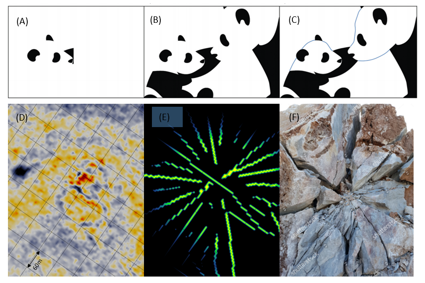
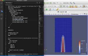
As a numerical modeler within the Seamstress team, my role is to simulate the effect of natural processes that could affects the regional stress field, by using advanced computational methods. The model presented here is a simulation of the Earth’s response to glaciation and deglaciation cycles, a physical process that is known as glacial isostatic adjustment (GIA). In other words, the Earth’s most outward layer, the lithosphere, falls or rises in reaction to its ice-age burden. In return, the deformation of the lithosphere results in the perturbation of the Earth’s stress field over regions affected by the glaciation and melting of the ice-sheet.

The following animation shows the magnitude of the maximum horizontal stress (SH) induced by GIA and calculated from the model for the last 122.8 kyrs. This period of time includes three episodes of glaciation and deglaciation that covers Greenland (Lecavalier et al., 2016), Fennoscandia, Svalbard and the Barents Sea (Patton et al., 2020). The ice models are applied at the surface of a spherical earth defined by a Maxwell viscoelastic rheology and includes every layers of the Earth from its surface to 2000 km depth.

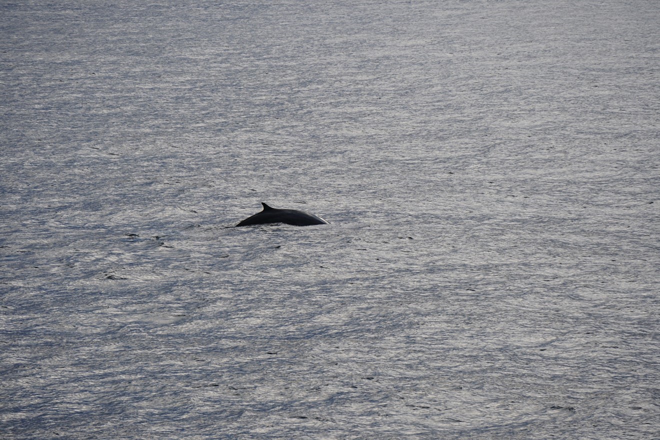
Results show that the maximum horizontal stresses are compressive in regions covered by ice and tensile off the edge of the ice-sheet. The local maximum of the horizontal stresses (around 30 MPa at the last glacial maximum for SH) matches with the ice thickness’s local maximum (around 3000 m at the last glacial maximum over Northern Sweden, Greenland and East of Svalbard). The tensile region located around the ice-sheet extent, results from the formation of a bulge that surrounds the subsidence zones formed by the weight of the ice cover on the Earth’s lithosphere. The pockmarks of Vestnesa ridge are located is a region where the forcing from the ice-sheet have probably influenced sediment fracturing as well as the  gas hydrate and free gas reservoir dynamics in this region.

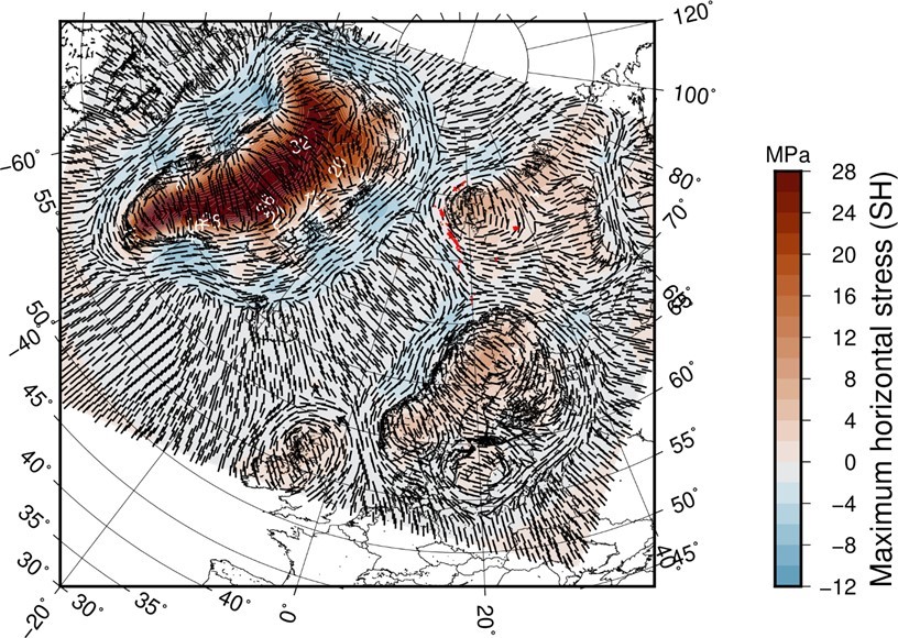
Figure: Map of maximum horizontal forcing (SH) derived from crustal adjustment following the retreat of the ice. Blue areas are subjected to a tensile stress regime whilst red areas are in a compressive stress regime. The black vectors indicate the orientation of the maximum horizontal stress.

 

Text and illustration Rémi Vachon

By the time the last Ocean Bottom Seismometer was diving deep into the ocean (previous post) big waves and strong winds arrived to us. We spent a day or so surviving to that feeling of sea sickness that accompanies you for a while even ashore…

Our next objective was to investigate how is the geology underlying the OBSs. For this the University vessel (Helmer Hanssen) is equipped with several instruments that produce and record acoustic waves of various frequencies. The lower the frequency of the wave the deeper we manage to image under the ground. But the higher the frequency, the more detail we get. We used every instrument available to get a highly detailed 3D image of the under-ground.

We collected geophysical data along 12 profiles and with the software onboard immediately produced spectacular “radiographies” of the mother Earth hidden under-water mountains and cracks in this remote part of the globe.

We started with 2D surveys (the ship moves in a straight line). Everything went so smooth and the excitement about amazing data was such, that we decided to do a 3D survey (the ship moves in parallel and closely spaced lines and the recorded data is then interpolated to get a volume).

Stormer and Steinar carefully connect the hydrophones to the cable that allows us to produce a 3D seismic image of the ground.

To image deeper we use an air source that produces an acoustic signal with 20-500 Hz. For 2D lines we connect the cables one after the other one (we refer to it as the green spaghetti).

The green spaghetti (the hydrophone cables) is rolled on deck while we change from 2D to 3D mode.

To image in 3D we put the cables one next to the other. Changing from one configuration to the other one implies a lot of action on deck for the crew, our engineers, ourselves and even our colleagues form AWI helped on deck pulling and connecting hydrophones for the surveys. Also the processing team had a lot of action and a sufficient amount of data to keep us awake during the night shifts.

Stormer and Steinar carefully dry and put leads in the hydrophone connectors while Henning and Vera (AWI) wait for the next hydrophone cable to role it into the box.

It was a productive research cruise with a great crew and lots of inspiring moments. We had intense research discussions and collected significant data sets for the Seamstress project. Part of the new lines complement as well a data set we are using for a scientific drilling proposal (IODP).

We sail satisfied to our next target before heading to our final destination…Home

Text and photos: Andreia Plaza-Faverola

We started the cruise being responsible with the law of the sea (we assisted a smaller ship that was in trouble). Luckily for the crew of the small ship and for ourselves, the weather was nice and the sea calm. So we collected the 7 seismometers (5 from Geomar, 2 from UiT) that were at the bottom since last year and started the next part of the experiment.

7 Ocean bottom seismometers from the Alfred Wegener Institute (AWI) waiting to go overboard. Photo by Andreia Plaza-Faverola

This time we left 10 seismometers at the bottom, 8 from AWI and 2 from UiT, distributed in a faulted region north of the Knipovich Ridge. In average the deployment of each instrument took about an hour. This included a test of the releasers (those we talked about in the first post of the expedition). The releasers were sent down to 2000 m inside a cage to check whether they were receiving the signal from the ship and responding with the task they were asked to do (open the hook!, close the hook!, send a signal back to the ship!, etc). Some of the releasers failed to obey in the last minute, almost like a child who refuses to do this and that. So they needed to be replaced (the releasers…). It was a long couple of days for all, in particular for those preparing the instruments to be thrown overboard.

Henning (AWI) observes and ensures the OBS is carefully driven to the sea surface by the crew member that operates the crane.  Photo by Andreia Plaza-Faverola 

Placing the instruments at sea went smooth. Now we all wait until next year to recover the instruments and hope they recorded small earthquakes originated or somehow related to faults that show up at the seafloor (along the so called passive continental margin) and that may be related to the opening of the Knipovich mid-Ocean ridge. Since shallow seismicity is not expected in the zone where the instruments sit (again, it is considered a “passive” continental margin slope), we can say in other words, we hope the instruments record something unexpected…

Towards the end the whales were still with us.

From left to right: an instrument, the crew and a whale.  Photo by Vera Schlindwein

 

 

 

Text by Andreia Plaza-Faverola

Photos by Vera Schlindwein and Andreia Plaza-Faverola

Seven ocean bottom seismometers (OBS) have been recording earthquakes for about a year at more than 1000 m water depth offshore the west-Svalbard margin. In a calm sea, surrounded by whales and dolphins we fished out one by one all of the instruments.

A porpoise swims around while we wait for a seismometer to show up at the horizon. Photo by Vera Schlindwein

Each seismometer is attached with a hook to an iron frame that keeps them on the sea-bottom over the recording period. To bring them back to the surface they are released from their weight using an acoustic device that sends a signal from the ship through the water, and basically tells the hook to rotate to leave the instrument free to float up. When one instrument is released we are all out at the bridge looking for it to show up at the horizon.

Przemek, Sunil and Stefan enjoy the calm sea while waiting for the instrument to appear at the surface

When the OBS is at the surface one of the crew fishes it out and grabs it with the crane or pick it up in the dingy.

To the left Jan throws the hook to fish the OBS so the crane can grab it. To the right, Stormer and Peter goes to pick an OBS that appeared farther away from the ship

Usually it takes about half an hour for one OBS to raise through 1200 m. There is always a latent fear of not getting the instruments back to the surface. But once again the operation was successful and we retrieved the 7 instruments.

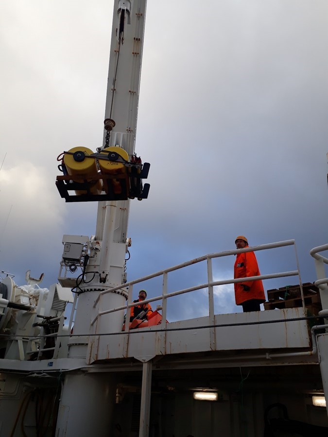
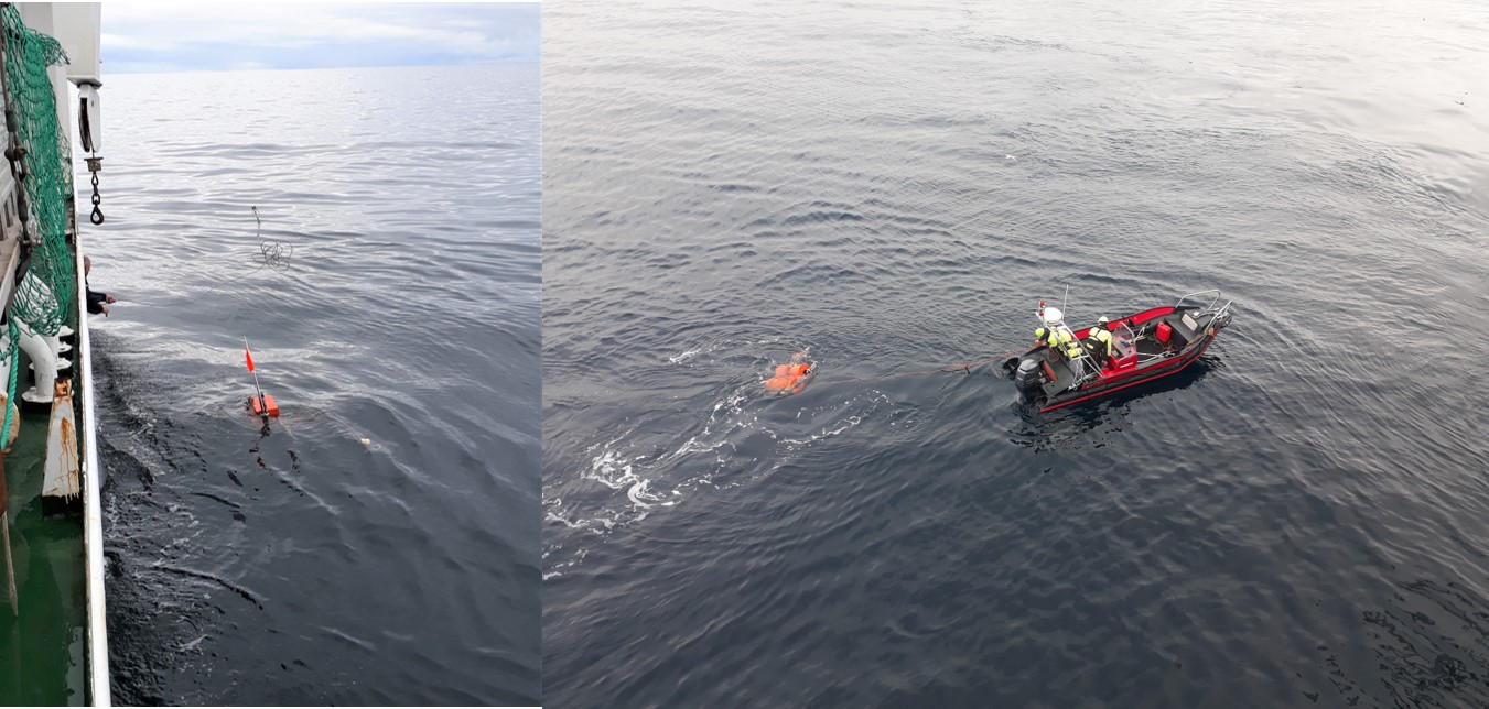
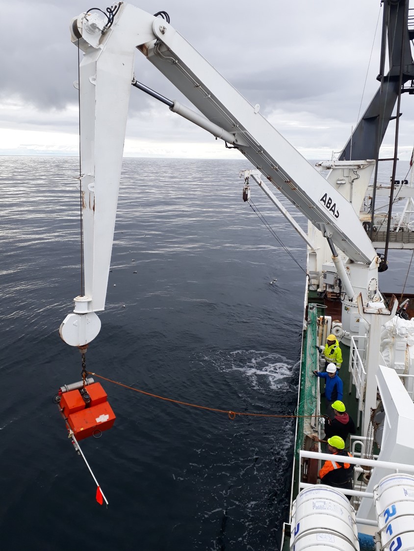
An OBS is taken from the sea back to the ship with the crane

Text and pictures by Andreia Plaza-Faverola

The second project expedition to continue with the Ocean Bottom Seismic (OBS) experiment started in Tromsø on the 19th of August 2020. This part of the experiment consists in collecting the seismometers that have been recording seismic signals since last summer around the Vestnesa Ridge (check previous posts), and placing new seismometers closer to the northern termination of the Knipovich mid-ocean ridge axis (check the map below). We are working closely with our colleagues from the Alfred Wegener Institute (AWI) in Germany. They bring the expertise on seismology as well as needed instrumentation.

The west-Svalbard continental margin is very close to the active mid-ocean ridge and it is thus a natural laboratory to study the impact of regional tectonic processes on shallow Earth processes such as the release of methane to the ocean.

The continental margins are classified as tectonically active (if one plate is colliding against another plate) or inactive (if the continental plate is far away from the middle of the oceans (mid-ocean ridges) where new rocks are being produced constantly). But what happens if a continental margin is not so far away from the mid-ocean ridges? This is what we are investigating. We are searching for small earthquakes along a margin that is supposed to be inactive (the west-Svalbard margin). The presence of earthquakes that originate at faults that are away from the mid-ocean ridge will indicate that the movement of oceanic plates at the mid-ocean ridges spreads to fractures and broken parts of the continental plate along the so called passive continental margins. Processes such as the release of methane to the oceans from these margins may be thus affected by tectonic movement from the oceanic ridges.

We have been transiting to the Fram Strait for about 48 hours already. Before starting with the OBS experiment we plan to collect seismic lines that are needed to complete a proposal for the International Ocean Discovery Program (IODP).

But not all is about pursuing scientific objectives. We are currently towing a small passenger boat that called for help because they got a rope (garbage floating in the ocean) entangled in their propeller. Our captain rescued them and will tow them until the coast guard takes over or until leaving them in a safe place. We needed to postponed the first surveys and adjust the schedule. Most likely we will need to reduce the amount of data we collect this time but we will take with us the good feeling of solidarity.

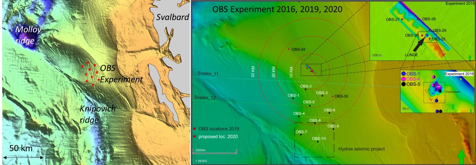
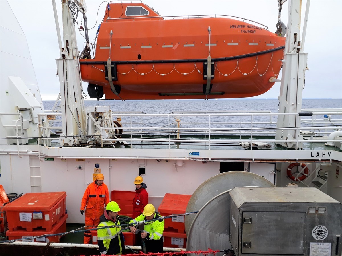
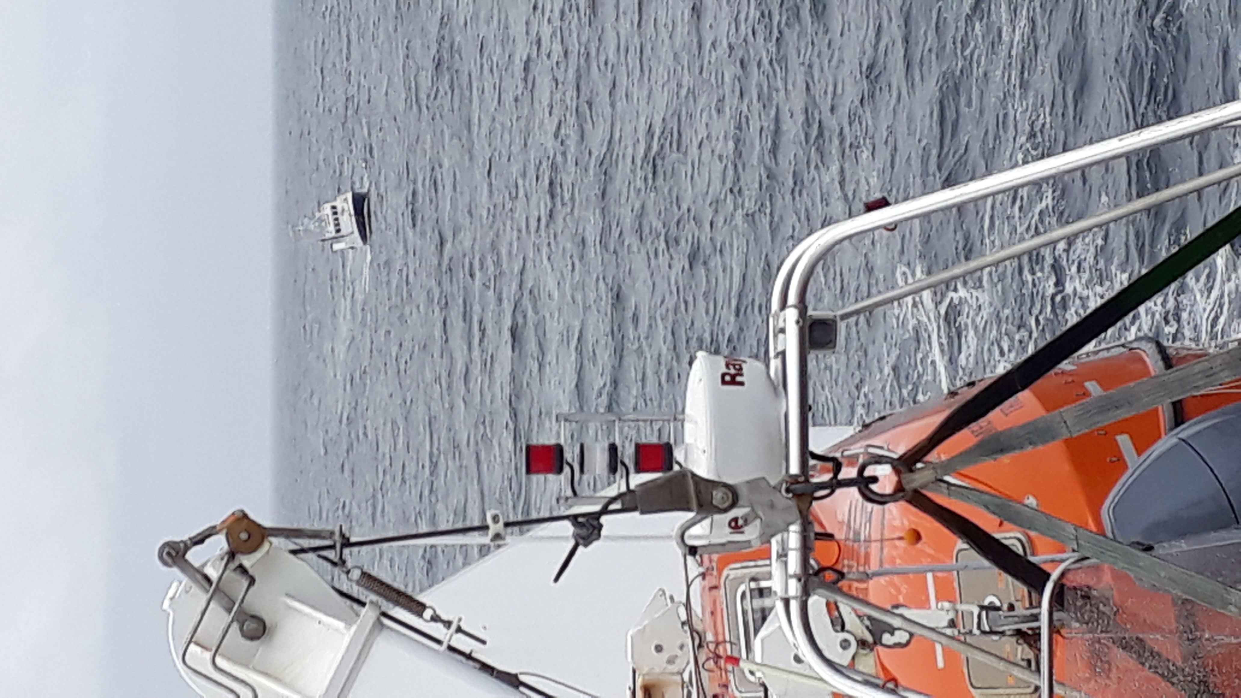
R/V Helmer Hanssen tows a small passenger ship in trouble to a safe place

Text: Andreia Plaza-Faverola

Figures: Przemek Domel, Sunil Vadakkepuliyambatta and Andreia Plaza-Faverola

Attributes describe seismic data. Seismic is a geophysical technique used to provide information about the subsurface using energy from sound. The technique requires no digging or drilling, but instead, uses a pulse of energy. The data recorded, is the time it takes for the energy emitted to bounce back from layers in the subsurface. Imagine an X-ray image of a slice of cake. This is close to the result!
Seismic attributes are prepared after seismic data collection. They reveal vital information about the seismic, quickly and effortlessly. The data is re-arranged through use of various calculations to help with pattern identification. It takes an experienced geologist or geophysicist to interpret the seismic attributes, as they are still ambiguous representations of the original data. Without the use of attributes, features in the original seismic data can be hidden. There are hundreds of different attributes available, and many of them reveal the same information. The key is choosing the right attribute or combination of attributes for the purpose of the task. It may take some time to find the right one, or combination of many, and you can easily get carried away with just wanting to try another to find an even better result! Attributes are extremely important for understanding seismic and for getting different views of your data, but you have to have an initial understanding of what you are looking for, to be able to choose the best attribute for your interpretation. The end goal is to have a more refined geological understanding of the subsurface. This of course will take some practice.
It is interesting to think about how we, as humans, process visual information. Our visual perception is largely influenced by context and colour. We have a cognitive ability to recognize patterns from what we see and relate them with past experience and knowledge (Paton and Henderson, 2015). For example, Figure 1 (A ): on first sight you see random, disparate shapes, but when the full image is revealed (B) it is then possible to interpret and draw in the missing sections of the image (C). This is context. We all know and recognize pandas! Imagine that the original seismic data (D) is, as though you are looking at the shapes in (A); that, the use of the correct attribute (E) has revealed (B) and that we, as experienced geological and geophysical interpreters, are able to draw the lines to reveal the deeper meaning of the original seismic (C). The lines could be important geological events for example, that were not obvious at first glance.
As a seismic interpreter, I am unable to see any meaningful information in the original seismic (D). Through applying calculations to the seismic data, by use of multiple seismic attributes, I have revealed much more information. I am able to see fractures radiating out from a central point (E). This however, may not be obvious to the non-seismic interpreter. Image (F) gives an alternative view. The photograph gives the viewer further context to understand what the attribute is showing. This is the bottom of a blasting hole, with fractures found in the rock after blasting. The hydro fracturing, as interpreted in (E) – thought to be a result of gas trapped in overpressured sediments – reveals the same fracture pattern as the blasting hole. The use of seismic attributes opens up the opportunity to investigate finer scale geological processes that may uncover details that could be the missing piece in the geological puzzle.

 

Figure 1 (A) – (C) from Paton and Henderson (2015), (D) original seismic, (E) seismic attribute, (F) from https://www.shutterstock.com/image-photo/bottom-blasting-hole-showing-fracture-rock-687006250

 

Text and illustration by Frances Cooke

Intuitively, you would assume that deep sea bottom is quiet, dead zone, devoid of activity. However, the reality is vastly different. When we drop seismometers to record what’s happening there, we pick up a lot of fascinating things. For the Seamstress project, we are putting seismometers on the bottom floor at more than 1000 m water depth along the west-Svalbard margin in the Fram Strait. We expected to listen and record earthquakes that can in turn give us information where tectonic plates press against each other, where they diverge and where slide in parallel. Since some of our observations took place in methane-seeping sites, we were hoping to record gas bubbling through the cracks in the seafloor, ultimately ending in hundreds-of-meter-long flares in the water column. And we got all of that. But we also recorded some other noise sources, trivial really. Only the biggest mammals that live in the world currently – the magnificent whales.

It is a tricky business to separate useful signal from the noise. However great and fascinating these creatures are (especially to biologists), they do not bring any information about subsurface that help geoscientists advance their understanding of underwater processes. Their very regular calls are often difficult to distinguish from, let’s say, signals that we interpret to be gas bubbling from the bottom of the sea.

One of the ideas to separate different sources is good, old Fourier transform. By assuming that what we recorded as one signal is really a combination of various frequencies, it is mathematically possible to separate all of them and visualize in the image called spectrum. We can then look at the portion of recording that we have doubts about and see what really it is consisting of.

On this image you can see what we think are separated fin and blue whale calls. While there is a great deal of studies related to recording their songs, each individual can have its own characteristic frequency range, making determination of the species difficult. It is a little easier to recognize fin whales, their regular song is usually a down-swept repeating signal in the frequency of 16-40 Hz that is dominating this image. But if you look closely at the 20 Hz, you can also see repeating, pulsating source, much weaker than the rest of the picture. There is a big chance that this is a call of blue whale, the largest mammal that ever existed.

It is fascinating to observe these calls, recognize different species and even track them using the direction of signal. When they are present in majority of your 10-month-long experiment designed to search for earthquakes and seepage however, they can become a bit of nuisance as well.

 

Text and illustration by Przemyslaw  Domel

In regard of the SEAMSTRESS project, a scientific cruise campaign (CAGE19-3) began Mid-October 2019 until beginning of November (3 weeks) in the Fram Strait, West of Svalbard. The objective of that cruise was to characterize the physical and geotechnical properties of sediments in the vicinity of pockmarks in the Vestnesa region. To do so, we sampled in-situ sediments by using a giant piston corer (core length = 10-20 m), a Gravity corer (core length = 3-6 m) and a Multi-Corer (core length = 1 m). Before and after the coring, a list of activities were performed by the science team on board, and later at the university facilities.

Orientation of Giant piston corer (GPC): For each deployment of the GPC, we installed a magnetic sensor upon the coring case in order to measure the orientation of the core. A first step of calibration was performed prior to the deployment of the magnetic sensor to estimate the location of the true North and magnetic North. This job was performed in collaboration with the ship crew and captain who provided us with the ship location and heading during the deployment of the GPC.

Geotechnical measurement on-board: After receiving, labeling and cutting the cores into 1-m long segments on deck, we performed a battery of geotechnical tests on the open sections such as: 1) shear strength, 2) density and 3) Water content measurements on the sediments.

Protocol for preparing the samples for geotechnical tests at NGI: In regard of the Seamstress project, we specifically stored vertically 15 sections (3 sections for each of the 5 targeted locations) that were chosen according to their depth and shear strength. Those sections were stored vertically to preserve the original conditions as much as possible and to avoid disturbing the sediment layers. Eight of those vertical sections have been sent to NGI in Oslo where they are being subjected to oedometer and triaxial tests (i.e., to study strain and derived-stress variations along the continental margin).

Lab work (MSCL and X-Ray): Once the cruise was over, further analysis were performed on the core sections in the NT-IG Laboratory. Every core collected during the expedition were thus scan by X-ray and multi-sensor core logger. Those profiles allow us to have a clear picture of the core and detailed data about the density, magnetic susceptibility and gamma ray of the sediments.

Subsampling for petrophysical analyses at the French Research Institute for Exploration of the Sea (IFREMER): In addition to sediment coring, in-situ pressure and temperature were measured using the piezometer instrument from IFREMER at 3 stations.  For further analysis of these data, a selection of sub-samples (depth and core section) were sent to IFREMER. Subsampling was made based on the depth of main anomalies along temperature and pressure logs from the piezometer. 10-cm long cylinders centered on the specific depths were prepared by looking at the CT scan images and processed MSCL logs.

Text and picture Rémi Vachon

Being part of Seamstress project means a lot of research. For a PhD, however it also means participation in courses in order to gather sweet ECTS points. My name is Przemek Domel and I work on marine seismology within Seamstress and CAGE. On March 1st I boarded the plane heading to Longyearbyen, „capital” of Svalbard archipelago, under Norwegian jurisdiction. My plan was simple – take part in Arctic Seismic Exploration course, meet new people and get hands on experience with acquiring data in harsh arctic conditions. Last, but not least, we were supposed to blow a lot of dynamite out (in the name of science, of course). First days did not  promise anything out of ordinary. I managed to greet and meet a lot of other students and a few PhDs, most of them originating from norwegian universities. We received proper training how to handle rifle (requirement for being outside city) and why snowmobiles are so much fun (they really are). I was very satisfied with the quality of lectures we started to receive prior to fieldwork and it looked that the course will be both memorable and valuable for my future work.

Stability is a fragile thing. As I was focusing on the task at hand, I paid less attention to the situation outside the Arctic. The world was slowly realizing that the new virus pandemic (Covid-19) has become a global threat, but at the time of my departure it looked that still only China and Italy were the countries truly affected and the situation was under control. So, last thursday, cut away from the news, I put as many layers of clothing as I could on myself in preparation of the first day of fieldwork (with the temperature on the glacier well below -30 degrees centigrade). But… it didn’t happen, first of all because it was too cold for the equipment to work and second because the scale of disease in Norway started to increase exponentially. We were sent to our dorms. Then the fieldwork was postponed. Then all the classes got cancelled. All within few hours. In the next two days information flow became chaotic, it was hard to realize whether the course will be taught at some later time, whether it is safer to stay in Svalbard than go back and whether we actually stay there. I am lucky to have very competent people to reach out for when I am in trouble. I was actually planning to stay for a little while and not pay for additional ticket, but my department leader Matthias and my supervisor Andreia suggested me coming back quickly due to volatility of situation and not worry about the costs. The same day I flew back, all of the students in Svalbard from outside Norway were forcibly evacuated to Oslo to protect the small community of Longyearbyen. Crazy times. But as a sun rose above the small city in arctic last week for the first time, I believe this crazy, cloudy period of history will come to an end soon as well.

Text and picture: Przemyslaw Domel

My name is Hariharan Ramachandran. I am a postdoc working in the seepage reconstruction task as part of the Project Seamstress. My major focus is to perform fluid flow simulations during methane venting at the Vestnesa Ridge. Specifically, the interdependence between the hydrate phase behavior and hydraulic fracturing during seepage. This task is performed in collaboration with Dr. Hugh Daigle, Associate Professor at the Petroleum and Geosystems Engineering, The University of Texas at Austin. I recently returned from 6-week trip in Texas. I focused on learning PFLOTRAN during my Austin stay as part of our collaboration. PFLOTRAN is a fully open-source subsurface flow and transport code with parallel computational capability. The capability to perform gas hydrate simulations was recently added to this model. This provides us an opportunity to investigate the seepage problem in 3D, which is particularly exciting. I spent my time learning how to setup a basic hydrate simulation problem and learning to use ParaView (open-source visualization software) to visualize results (Fig 1). On the other side, I got an opportunity to revisit my alma mater, meet old friends, and relax at my favorite haunts in Austin. After completing a 5-week stay at Austin, I visited Galveston, Houston to attend the natural gas hydrates systems section of Gordon Research Seminar. I presented (~15mins talk) about the Project Seamstress and the seepage-modeling task to the gas hydrates community.

Fig 1: Example workspace. The window on the left shows a typical pflotran input file in VS CODE editor. The window on the right shows the output visualization in ParaView.

By Hariharan Ramachandran